Tutorial 1: R, syntax, atomic elements and console.
Introduction
To encourage new users, the purpose of these tutorials is to to teach you Data Science using the R-language in the simplest way . Learning Data Science goes hand in hand with gaining skills with a computer programming language. As it was covered in the first lecture, R is a free open source language
I have identified, through my experience of teaching R, six main building blocks of the language. We will cover these blocks in the following way:
- Week 1: Learn R and its integration with R-studio, the operators, the atomic element and basic operations in the console.
- Week 2: Learn basic
objectcreation and manipulation:vectors,matrices,dataframes,arrays,lists. - Week 3: How to read/save data from R, and how to perform descriptive statistics and linear regression.
- Week 4: Basic Data Visualization Using R.
- Week 5: Basic Algorithms 1: Use of
functions,loops,while,if,elsestatements. - Week 6 onward, we will deploy our skill running Machine Learning (ML) algorithms and String Analysis.
Instroctutions for the tutorials.
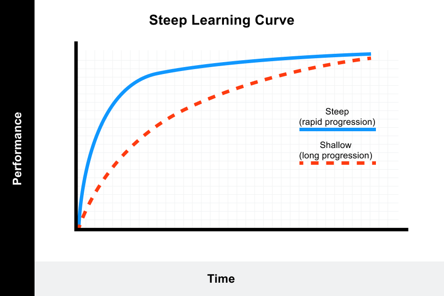
The exercises are simple, designed to develop intuition, confidence to step the learning curve!
Source: Valamis, 2020
- Each weak, you will take look in this repository and read the corresponding tutorial exercise for each week.
- Here in this website, I am posting the instructions and the solutions to all the exercises.
- Your task is to perform all the excercises of each tutorial in an
Rscrip, you can download the template. - Here you can see an example of what to do in each tutorial:
 Tip: If the image is too small, download it, and view in your
computer.
Tip: If the image is too small, download it, and view in your
computer.
The R operators
The operators are special characters that perform an action with
a specific result. The most common arithmetic operators to get some
familiarity. These operators are not only common for R but you may
know them from spreadsheets, calculators or other languages.
CRAN has an exhaustive list of operators that you can retrieve here
| List of Operators | |
|---|---|
| - | Minus. |
| + | Plus. |
| : | Sequence. |
| * | Multiplication. |
| / | Division. |
| ^ | Exponentiation. |
| %% | Modulus. |
Atomic elements.
The atomic elements are the most fundamental building blocks of the R language. They are the most essential input of the language, here are the main types:
| Atomic Element | |
|---|---|
| 1L, 2L, 3L, 10L | Integer. |
|
1.1, 4.5, 3.2 |
Numeric. |
| “A”, “B”,“3” | Character. |
|
TRUE, FALSE |
Logical. |
|
NA |
Not Available / Missing Values. |
Lines and chunks of code.
Now we can use operators + atomic elements to write lines of code. R runs these lines of code following these two rules:
- Similar to math, lines are read and evaluated from left to right.
- Similar to a book, lines are read and evaluated from top to button.
Lines of code are used to perform analysis, evaluate statements and any
sort of operation that you can imagine. Different from independent lines
of code, a group of two or more lines used for a particular operation is
called a chunk of code. But, before we get into them, practice your
knowledge of operators and atomic elements to perform basic arithmetic
operations.
Other resources:
If you want to increase your knowledge of R and accelerate your learning check out:
- The excellent Introduction to R from Datacamp.
- The Comprehensive R Archive Network (CRAN) also has a more comprehensive manual.
- Watch for free the videos of the Advance Your Skills as an R Expert, from Linkedin
Exercise 1: Use R as a calculator.
Instruction: Solve the following exercises by writing the correct atomic elements and operators to perform each arithmetic operation. Each exercise can solve in different ways, but the solution should be the same.
Writing tips
- Use the most simple combination of atomic elements and
operators. For instance, if asked to perform
2 plus 3, avoid using more atomic elements and operators typing2 + 1 + 1 + 1. The best answer is not only correct but also the simplest. Example:2 + 3. - Leave a space or white space in between each operator and atomic
element. For instance, write
2 + 3but not2+3. An exception to this rule is to write powers, which3^3is preferred but not
Solve:
- 1.1 Addition: 2 plus 3.
[1] 5
- 1.2 Subtraction: 5 minus 4. 5 - 4
[1] 1
- 1.3 Multiplication: 3 times 5.
[1] 15
- 1.4 Division: 10 divided by 2.
[1] 5
- 1.5 Exponentiation: 4 to the power of 3.
[1] 64
- 1.6 Module: 5 module 2
[1] 1
Exercise 2: Use of parentheses.
Use parentheses () to group expressions only if needed. For instance,
(3 + 2) is equivalent to 2 + 3, but the latter answer uses fewer
operators, and it is better. Parentheses are used correctly to specify
the order in which R performs operations. For instance, 9 + 1/2 is
not the same as (9 + 1)/2. In the former expression, 9 is added to
1/2, but in the latter (9 + 1) is solved first and then divided
(9 + 1)/2. Remember that lines are evaluated from left to right.
- 2.1 Solve 10 plus 5 and divide by 3. Hint solution is 5.
(10 + 5)/3
[1] 5
Solve, the next exercises:
- 2.2 Solve 6 plus 3 to the power of 2 and divide by 3. Hint, the solution is 27.
[1] 27
- 2.3 Solve 16 to the power of 1/2 multiplied by 3. Hint, the solution is 24.
[1] 24
- 2.4 Multiply 3 times 12 plus 4, all divided by 2. Hint, the solution is 24.
[1] 24
- 2.5 Divide 4 by 2 times 3, all that times 18 minus 6. Hint, the solution is 8
[1] 8
Exercise 3: Use of logical operators
The logical operators is used to assess relationships between atomic elements. Here you have some examples:
- The snipped
4==4, will return aTRUEin the console. - The snipped
4==3, will return aFALSEin the console. - The snipped
7!=7, will return aFALSEin the console because7is not different from7. - The snipped
5>3, will return aFALSE. - Similarly,
5<7, will return aFALSE. - But not,
2<=4, that will returnTRUE, because2is smaller or equal to4
Solve:
- 3.1 Assess if TRUE is equal to TRUE, and then to FALSE. Tip, you have to group using parenthesis.
(T == T) == F
[1] FALSE
- 3.2 Verify if 4 is greater than 6.
[1] FALSE
- 3.3 Verify that 7 is less than 2.
[1] FALSE
- 3.4 Verify that 6 times 7 is less than 8 times 9.
[1] FALSE
- 3.5 Vecorized: Evaluates element by element. DO NOT CHANGE THE CODE!
c(2, 3, 4) | c(2, 3, 4) == c(2, 3, 4)
[1] TRUE TRUE TRUE
- 3.6 Not vectorlized: outputs a single statement. DO NOT CHANGE THE CODE!
c(2, 3, 4) || c(2, 3, 4) == c(2, 3, 4)
[1] TRUE
Excersise 4: Objects
R is an object-oriented programming language, which means for simplicity that everything aside the operators and syntax is defined an object.
This objects have specific attributes which can be retrieved by
functions, such as: class class(x), structure str(x); type of
typeof(x). Unidimensional objects such as vectors and lists are
compatible with the length(x) which returns their number of elements
for instance. However, more complex objects (multidimensional), such as
matrices and data frames have dimensions, returned by dim(x), also
nrow(x) and ncol(x) to estimate the number of rows and columns
respectively.
Pay attention to the use of the left assignment <- for storing
objects; the parenthesis () for declaring arguments of functions;
and squared brakets [] or the dollar sign $ for subsetting
objects.
Vectors (Also called atomic vectors).
Sole:
- 4.1 Declare a
NULLvector calledz, then assess theclass,lengthandtypeofobject.
[1] "NULL"

[1] 0

[1] "NULL"
- 4.2 Declare a
numericvectorwith two elementsc(1,2)calleda. Then, add namesc('one', 'two')to the elements ofawith thenamesfunction. Print thenamesofa.
[1] "one" "two"
- 4.3 Extract the element of
acalledtwoand print the output in the console.
two
  2
- 4.4 Create a
vectorwith two integers, remember to use theLoperator after the number. For instance,1L, but not1. Call this vector `band print theclassin the console.
[1] "integer"
- 4.5 Create a logical vector with two elements
c(T, F), call this vectorc. Then use this vector to print the vectorbin the console.
[1] 2
- 4.6 Use the function
LETTERSto create acharactervectorwith the first 10 letters of the alphabet. Call this vectordand print it in the console.
[1] "A" "B" "C" "D" "E" "F" "G" "H" "I" "J"
- 4.7 Create a
factorcallede, which is a categorical variable, with two elementsc('male', 'female')with the functionfactor, print theclassof vector in the console.
[1] "factor"
- 4.8 Create an ordinal variable with the function
factorcalledf, with thelabelsc('poor', 'good', 'excellent'); print thevectorand check thatis.orderedreturns aTRUEvalue.
[1] poor      good      excellent
Levels: poor < good < excellent

[1] TRUE
Matrices, Data Frames and Lists.
- 5.1 Create a
matrixof5x5with the numbers from1Lto25L. Put the element in ascendant order in everyrowand call it this matrixA, print it in the console.
     [,1] [,2] [,3] [,4] [,5]
[1,]    1    2    3    4    5
[2,]    6    7    8    9   10
[3,]   11   12   13   14   15
[4,]   16   17   18   19   20
[5,]   21   22   23   24   25
- 5.2 Use the function
rbindto arrange threecharactervectorswith two elements each by row. Call this matrixBand print it in the console.
  [,1] [,2]
a "A"  "B"
b "C"  "D"
c "E"  "F"
- 5.3 Assess the class of matrices
AandB, print the output in the console.
[1] "matrix" "array"

[1] "matrix" "array"
- 5.4 Extract the 25th element of the matrix
A, print the output in the console.
[1] 25
- 5.5 Extract the second column of the matrix
Band print it in the console.
  a   b   c
"B" "D" "F"
- 5.6 Transform the matrix
Ainto adata.frameand call itdf1, print thedim, dimmension, of this object.
[1] 5 5
- 5.7 Create 5 vectors,
integer,numeric,logical,characterandfactor, call this vectorsa,b, …,e, with three elements respectively. Then use this vectors to create adata.framewith five columns, one for each vector. Call this last objectdf2and print the output in the console.
  a  b     c d e
1 1  6  TRUE k P
2 2  7 FALSE l Q
3 3  8  TRUE m R
4 4  9 FALSE n S
5 5 10 FALSE o T
- 5.8 Assess the
classof each column of thedf2and print the output in the console.
$a
[1] "integer"

$b
[1] "integer"

$c
[1] "logical"

$d
[1] "character"

$e
[1] "factor"
- 5.9 Create a list, called
L1, that contains matricesA,B, and the data framesdf1anddf2, and the vectorsb,cande. Print the output in the console.
[[1]]
     [,1] [,2] [,3] [,4] [,5]
[1,]    1    2    3    4    5
[2,]    6    7    8    9   10
[3,]   11   12   13   14   15
[4,]   16   17   18   19   20
[5,]   21   22   23   24   25

[[2]]
  [,1] [,2]
a "A"  "B"
b "C"  "D"
c "E"  "F"

[[3]]
  V1 V2 V3 V4 V5
1  1  2  3  4  5
2  6  7  8  9 10
3 11 12 13 14 15
4 16 17 18 19 20
5 21 22 23 24 25

[[4]]
  a  b     c d e
1 1  6  TRUE k P
2 2  7 FALSE l Q
3 3  8  TRUE m R
4 4  9 FALSE n S
5 5 10 FALSE o T

[[5]]
[1]  6  7  8  9 10

[[6]]
[1]  TRUE FALSE  TRUE FALSE FALSE

[[7]]
[1] P Q R S T
Levels: P Q R S T
Excersise 6: Theoretical Questions.
-
6.1 How does Data Science is different from statistics and mathematics?
-
6.2 Explain one advantage of Big data in comparison to survey data or experimental data.
-
6.3 Explain the main activities in Data Science that take place before the analysis.